Techniques of Demand Forecasting (Survey and Statistical Methods)

The main challenge to forecast demand is to select an effective technique.

There is no particular method that enables organizations to anticipate risks and uncertainties in future. Generally, there are two approaches to demand forecasting.

The first approach involves forecasting demand by collecting information regarding the buying behavior of consumers from experts or through conducting surveys. On the other hand, the second method is to forecast demand by using the past data through statistical techniques.

Thus, we can say that the techniques of demand forecasting are divided into survey methods and statistical methods. The survey method is generally for short-term forecasting, whereas statistical methods are used to forecast demand in the long run.

These two approaches are shown in Figure-10:

Let us discuss these techniques (as shown in Figure-10).

Survey Method:

Survey method is one of the most common and direct methods of forecasting demand in the short term. This method encompasses the future purchase plans of consumers and their intentions. In this method, an organization conducts surveys with consumers to determine the demand for their existing products and services and anticipate the future demand accordingly.

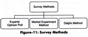
The survey method undertakes three exercises, which are shown in Figure-11:

The exercises undertaken in the survey method (as shown in Figure-11) are discussed as follows:

i. Experts’ Opinion Poll:

Refers to a method in which experts are requested to provide their opinion about the product. Generally, in an organization, sales representatives act as experts who can assess the demand for the product in different areas, regions, or cities.

Sales representatives are in close touch with consumers; therefore, they are well aware of the consumers’ future purchase plans, their reactions to market change, and their perceptions for other competing products. They provide an approximate estimate of the demand for the organization’s products. This method is quite simple and less expensive.

However, it has its own limitations, which are discussed as follows:

a. Provides estimates that are dependent on the market skills of experts and their experience. These skills differ from individual to individual. In this way, making exact demand forecasts becomes difficult.

b. Involves subjective judgment of the assessor, which may lead to over or under-estimation.

c. Depends on data provided by sales representatives who may have inadequate information about the market.

d. Ignores factors, such as change in Gross National Product, availability of credit, and future prospects of the industry, which may prove helpful in demand forecasting.

ii. Delphi Method:

Refers to a group decision-making technique of forecasting demand. In this method, questions are individually asked from a group of experts to obtain their opinions on demand for products in future. These questions are repeatedly asked until a consensus is obtained.

In addition, in this method, each expert is provided information regarding the estimates made by other experts in the group, so that he/she can revise his/her estimates with respect to others’ estimates. In this way, the forecasts are cross checked among experts to reach more accurate decision making.

Ever expert is allowed to react or provide suggestions on others’ estimates. However, the names of experts are kept anonymous while exchanging estimates among experts to facilitate fair judgment and reduce halo effect.

The main advantage of this method is that it is time and cost effective as a number of experts are approached in a short time without spending on other resources. However, this method may lead to subjective decision making.

iii. Market Experiment Method:

Involves collecting necessary information regarding the current and future demand for a product. This method carries out the studies and experiments on consumer behavior under actual market conditions. In this method, some areas of markets are selected with similar features, such as population, income levels, cultural background, and tastes of consumers.

The market experiments are carried out with the help of changing prices and expenditure, so that the resultant changes in the demand are recorded. These results help in forecasting future demand.

There are various limitations of this method, which are as follows:

a. Refers to an expensive method; therefore, it may not be affordable by small-scale organizations

b. Affects the results of experiments due to various social-economic conditions, such as strikes, political instability, natural calamities

Statistical Methods:

Statistical methods are complex set of methods of demand forecasting. These methods are used to forecast demand in the long term. In this method, demand is forecasted on the basis of historical data and cross-sectional data.

Historical data refers to the past data obtained from various sources, such as previous years’ balance sheets and market survey reports. On the other hand, cross-sectional data is collected by conducting interviews with individuals and performing market surveys. Unlike survey methods, statistical methods are cost effective and reliable as the element of subjectivity is minimum in these methods.

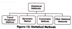
These different statistical methods are shown in Figure-12:

The different statistical methods (as shown in Figure-12).

Trend Projection Method:

Trend projection or least square method is the classical method of business forecasting. In this method, a large amount of reliable data is required for forecasting demand. In addition, this method assumes that the factors, such as sales and demand, responsible for past trends would remain the same in future.

In this method, sales forecasts are made through analysis of past data taken from previous year’s books of accounts. In case of new organizations, sales data is taken from organizations already existing in the same industry. This method uses time-series data on sales for forecasting the demand of a product.

Table-1 shows the time-series data of XYZ Organization:

The trend projection method undertakes three more methods in account, which are as follows:

i. Graphical Method:

Helps in forecasting the future sales of an organization with the help of a graph. The sales data is plotted on a graph and a line is drawn on plotted points.

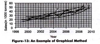
Let us learn this through a graph shown in Figure-13:

Figure-13 shows a curve which is plotted by taking into the account the sales data of XYZ Organization (Table-1). Line P is drawn through mid-points of the curve and S is a straight line. These lines are extended to get the future sales for year 2010 which is approximately 47 tons. This method is very simple and less expensive; however, the projections made by this method may be based on the personal bias of the forecaster.

ii. Fitting Trend Method:

Implies a least square method in which a trend line (curve) is fitted to the time-series data of sales with the help of statistical techniques.

In this method, there are two types of trends taken into account, which are explained as follows:

a. Linear Trend:

Implies a trend in which sales show a rising trend.

In linear trend, following straight line trend equation is fitted:

S = A+BT

Where

S= annual sales

T=time (in years)

A and B are constant

B gives the measure of annual increase in sales

b. Exponential Trend:

Implies a trend in which sales increase over the past years at an increasing rate or constant rate.

The appropriate trend equation used is as follows:

Y = aT^b

Where

Y= annual sales

T= time in years

a and b are constant

Converting this into logarithm, the equation would be:

Log Y = Log a + b Log T

The main advantage of this method is that it is simple to use. Moreover, the data requirement of this method is very limited (as only sales data is required), thus it is inexpensive method.

However, this method also suffers from certain limitations, which are as follows:

1. Assumes that the past rate of changes in variables will remain same in future too, which is not applicable in the practical situations.

2. Fails to be applied for short-term estimates and where trend is cyclical with lot of fluctuations

3. Fails to measure relationship between dependent and independent variables.

iii. Box-Jenkins Method:

Refers to a method that is used only for short-term predictions. This method forecasts demand only with stationary time-series data that does not reveal the long-term trend. It is used in those situations where time series data depicts monthly or seasonal variations with some degrees of regularity. For instance, this method can be used for estimating the sales forecasts of woolen clothes during the winter season.

Barometric Method:

In barometric method, demand is predicted on the basis of past events or key variables occurring in the present. This method is also used to predict various economic indicators, such as saving, investment, and income. This method was introduced by Harvard Economic Service in 1920 and further revised by National Bureau of Economic Research (NBER) in 1930s.

This technique helps in determining the general trend of business activities. For example, suppose government allots land to the XYZ society for constructing buildings. This indicates that there would be high demand for cement, bricks, and steel.

The main advantage of this method is that it is applicable even in the absence of past data. However, this method is not applicable in case of new products. In addition, it loses its applicability when there is no time lag between economic indicator and demand.

Econometric Methods:

Econometric methods combine statistical tools with economic theories for forecasting. The forecasts made by this method are very reliable than any other method. An econometric model consists of two types of methods namely, regression model and simultaneous equations model.

These two types of methods are explained as follows:

i. Regression Methods:

Refer to the most popular method of demand forecasting. In regression method, the demand function for a product is estimated where demand is dependent variable and variables that determine the demand are independent variable.

If only one variable affects the demand, then it is called single variable demand function. Thus, simple regression techniques are used. If demand is affected by many variables, then it is called multi-variable demand function. Therefore, in such a case, multiple regression is used.

The simple and multiple regression techniques are discussed as follows:

a. Simple Regression:

Refers to studying the relationship between two variables where one is independent variable and the other is dependent variable.

The equation to calculate simple regression is as follows:

Y = a + bx

Where, Y = Estimated value of Y for a given value of X

b = Amount of change in Y produced by a unit change in X

a and b = Constants

The equations to calculate a and b are as follows:

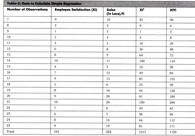
Let us learn to calculate simple regression with the help of an example. Suppose a researcher wants to study the relationship between the employee (sales group) satisfaction and sales of an organization.

He/she has taken the feedback from the employees in the form of questionnaire and asked them to rate their satisfaction level on a 10-pointer scale where 10 is the highest and 1 is the lowest. The researcher has taken the sales data for every individual member of the sales group. He/she has taken the average of monthly sales for an year for every individual.

The collected data is arranged in Table-2:

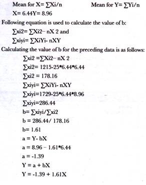
The calculation of mean for employee satisfaction (X) and sales is as follows:

This is the regression equation in which the researcher can take any value of X to find the estimated value of Y.

For example, if the value of X is 9, then the value of Y would be calculated as follows:

Y = -1.39 + 1.61X

Y = -1.39 + 1.61(9)

Y= 13.1

With the help of preceding example, it can be concluded that if an employee is satisfied, then his/her output would increase.

b. Multiple Regression:

Refers to studying the relationship between more than one independent and dependent variables.

In case of two independent variables and one dependent variable, following equation is used to calculate multiple regression:

Y = a + b1X1 +b2X2

Where, Y (Dependent variable) = Estimated value of Y for a given value of X1 and X1

X1 and X2 = Independent variables

b1 = Amount of change in Y produced by a unit change in X1

b2 = Amount of change in Y produced by a unit change in X2

a, b1 and b2 = Constants

The equations used to calculate a and b values are as follows:

The number of equations depends on the number of independent variables. If there are two independent variables, then there would be three equations and so on.

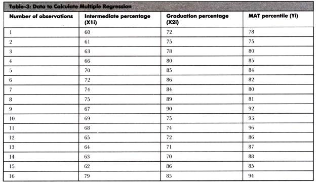
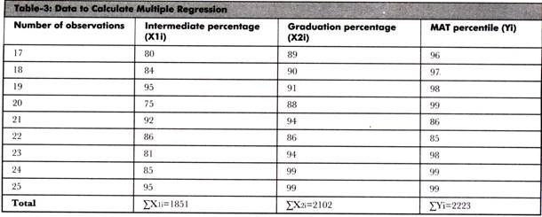
Let us learn to calculate multiple regression with the help of an example. Suppose the researcher wants to study the relationship between intermediate percentage, graduation percentage, and MAT percentile of a group of 25 students.

It is important to note that intermediate percentage and graduation percentage are independent variables and MAT percentile is dependent variable. The researcher wants to find out whether the percentile in MAT depends on the percentage of intermediate and graduation or not.

The collected data is shown in Table-3:

The equations required to calculate multiple regression are as follows:

These equations are used to solve the multiple regression equation manually. However, you can also use SPSS to find out multiple regression.

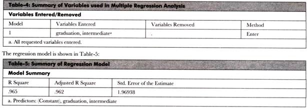
If we use SPSS in the preceding example, we would get the output shown in Table-4:

Table-5 shows the summary of the regression model. In this table, R is the correlation coefficient between the independent and dependent variables, which is very high in this case. R Square shows that a large part of variation in the model is shown by employment opportunities in a state. Standard error of estimate is quite low that is 1.97. It also indicates that the variation in the present data is less.

Table-6 shows the coefficients of regression model:

Table-6 shows that the calculated t value is greater than the significance t value. Thus, the coefficients show cause and effect relationship between the independent and dependent variables.

Table-7 shows the AN OVA table for the two variables under study:

Table-7 shows the analysis of variation in the model. The regression row shows the variation occurred due to regression model. However, the residual row shows the variation that occurred by chance. In Table-7, the value of sum of squares for regression row is greater than the value of sum of squares for residual row; therefore, most of the variations are produced only due to model.

The calculated F value is very large as compared to the significance value. Therefore, we can say that the intermediate percentage and graduation percentage have a strong effect on the MAT percentile of a student.

Simultaneous Equations:

Involve several simultaneous equations.

There are two types of variables that are included in this model, which are as follows:

i. Endogenous Variables:

Refer to inputs that are determined within the model. These are controlled variables.

ii. Exogenous Variables:

Refer to inputs of the model. Examples are time, government spending, and weather conditions. These variables are determined outside the model.

For developing a complete model, endogenous and exogenous variables are determined first. After that, necessary data on both exogenous and endogenous variables are collected. Sometimes, data is not available in required form, thus, it needs to be adjusted into the model.

After the development of necessary data, the model is estimated through some appropriate method. Finally, the model is solved for each endogenous variable in terms of exogenous variable. The prediction is finally made.

Other Statistical Measures:

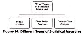
Apart from statistical methods, there are other methods for demand forecasting. These measures are very specific and used for only particular datasets. Therefore, there usage cannot be generalized for all types of research.

These measures are shown in Figure-14:

The different types of statistical measures (as shown in Figure-14) are discussed as follows:

iii. Index Number:

Refers to the measures used to study the fluctuations in a variable or group of related variables with respect to time period/base period. They are most commonly used in economics and financial research to study various factors, such as price and quantity of a product. The factors that are responsible for the problem are identified and calculated.

There are mainly four types of index numbers, which are as follows:

a. Simple index number:

Refers to the number that measures a relative change in a single variable with respect to the base year.

b. Composite index number:

Refers to the number that measures a relative change in a group of related variables with respect to the base year.

c. Price index number:

Refers to the number that measures a relative change in the price of a commodity in different time periods.

d. Quantity index number:

Refers to the number that measures a relative change in the physical quantity of goods produced, consumed or sold for a commodity in different time periods.

Time Series Analysis: Refers to the analysis of a series of observations over a period of equally spaced time intervals. For example analyzing the growth of a company from its incorporation to the present situation. Time series analysis is applicable in various fields, such as public sector, economics, and research.

There are various components of time series analysis, which are as follows:

a. Secular Trend:

Refers to the trend that is denoted by T and prevalent over a period of time. Secular trend for a data series can be upward or downward. The upward trend shows the increase in a variable, such as increase in prices of commodities; whereas, the downward trend shows the declining phases, such as decline in the rate of diseases and sales for a particular product.

b. Short Time Oscillation:

Refers to a trend that remains for a shorter period of time.

It can be classified into the following three trends:

1. Seasonal trend:

Refers to the trend that is denoted by S and occurs year after year for a particular period. The reason for such trends is weather conditions, festivals, and some other customs. Examples of seasonal trend are the increase in the demand for woolens in winters and increase in sales for sweet near Diwali.

2. Cyclical Trend:

Refers to the trend that is denoted by C and lasts more than for an year. Cyclical trends are neither continuous nor seasonal in nature. An example of cyclical trend is business cycle.

3. Irregular trend:

Refers to the trend that is denoted by I and is short and unpredictable in nature. Examples of irregular trends are earthquakes, volcano eruptions, and floods.

Decision Tree Analysis:

Refers to the model that is used to take decision in an organization. In the decision tree analysis, a tree-type structure is drawn to decide the best solution for a problem. In this analysis, we first find out different options that we can apply to solve a particular problem.

After that, we can find out the outcome of each option. These options/decisions are connected with a square node while the outcomes are demonstrated with a circle node. The flow of a decision tree should be from left to right.

The shape of the decision tree is shown in Figure-15:

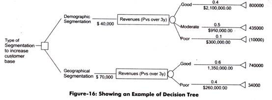
Let us understand the working of a decision tree with the help of an example. Suppose an organization wants to decide the type of segmentation to increase the customer base.

This problem can be solved by using the decision tree shown in Figure-16:

In Figure-16, the decision tree shows two types of segmentation, namely demographic segmentation and geographical segmentation. Now, we would analyze the outcomes of these two segmentations. To analyze the demographic segmentation, the company has to incur S 40,000 (estimated cost). The outcome of the demographic segmentation can be good, moderate, and poor.

The estimated revenue projected for three years for the three options (good, moderate, and poor) are as follows:

Good = $ 21500000

Moderate = $ 950000

Poor= S300000

The probabilities assigned to the outcomes are 0.4 for good, 0.5 for moderate, and 0.1 for poor.

Now, we calculate the outcomes of demographic segmentation in the following manner:

Good= 0.4*2100000 = 840000

Moderate = 0.5*950000=475000

Poor = 0.1*300000= 30000

Similarly, in case of geographical segmentation, the cost incurred is $ 70000 (estimated cost). The outcome of the geographical segmentation can be good and poor.

The estimated revenue projected for three years for the two options (good and poor) are as follows:

Good = $ 1350000

Poor= $ 260000

The probabilities assigned to the outcomes are 0.6 for good and 0.4 for poor.

Now, we calculate the outcomes of geographical segmentation in the following manner:

Good= 0.6*1350000 = $ 810000

Poor = 0.4*260000 = $ 104000

Now, we would analyze the two outcomes for taking a decision to select one segmentation out of the two segmentations in the following manner:

For demographic segmentation:

Good= 840000-40000= $ 800000

Moderate = 475000-40000= $ 435000

Poor = 30000-40000= $ (10000)

Similarly, for geographical segmentation:

Good= 810000-70000= $ 740000

Poor =104000-70000= $ 340000

As we can see from the calculation that if we select the demographic segmentation, then the maximum estimated profit would be $ 800000. In demographic segmentation, there are chances of incurring losses (10,000), if the product is not successful in the market.

If we select geographical segmentation, then the maximum estimated profit would be$ 740000. In geographical segmentation, we would earn less profit (S 340000), if the product is not successful in the market. Therefore, it is better to use geographical segmentation for marketing the product, as no loss is involved in it.